Interpretability of the image quality metrics¶

Tutorial.

MRIQC provides a comprehensive framework for assessing the quality of MR images in research studies. Alongside its visual reports, it generates a large collection of Image Quality Metrics (IQMs) that quantify different aspects of image integrity. While this breadth of information is valuable, the sheer number of available metrics can make it challenging for researchers to determine which IQMs are most informative when judging the quality of a specific image. Clear guidance on which metrics to prioritize can help streamline quality assessment and support more consistent decision‑making across studies.

Data¶

The T1w IQMs used in this analysis were downloaded from the MRIQC Quality Control REST API:

https://mriqc.nimh.nih.gov/api/v1/T1w

This endpoint provides community‑contributed Image Quality Metrics (IQMs) for T1‑weighted structural MRI scans, enabling comparisons against large normative datasets.

import brainprep
import numpy as np
import pandas as pd
from pathlib import Path


resource_dir = Path(brainprep.__file__).parent / "resources"
data_df = pd.read_csv(resource_dir / "iqm_T1w.csv")
columns = [
    name
    for name in data_df.columns
    if not name.startswith(("provenance.", "bids_meta.", "size_", "spacing_",
                            "summary_", "tpm_"))
]
data_df = data_df[sorted(columns)]
iqms = data_df.drop([
    "_created",
    "_etag",
    "_id",
    "_links.self.href",
    "_links.self.title",
    "_updated"
], axis=1)
print(iqms)

          cjv       cnr       efc  ...  snrd_total    snrd_wm    wm2max
  0.723938  1.858954  0.564140  ...   34.839946  48.247816  0.547152
  0.852123  1.508577  0.738258  ...    7.894523  10.766795  0.418142
  0.560600  2.448116  0.563207  ...   43.914040  62.502591  0.706322
  0.793762  1.694586  0.572623  ...   30.201655  41.838399  0.652624
  0.760221  1.715271  0.674800  ...   10.116118  13.589410  0.387541
..        ...       ...       ...  ...         ...        ...       ...
0.516082  2.383230  0.614017  ...   14.102988  20.393643  0.665563
0.482430  2.603823  0.616080  ...   18.119880  24.867607  0.657314
0.733260  1.699137  0.674015  ...   10.904249  15.278017  0.588805
0.393971  3.029418  0.583193  ...   19.960742  29.703942  0.675711
0.699660  1.854568  0.648808  ...   12.753427  18.473011  0.614847

[1000 rows x 27 columns]

Data scaling¶

Normalizing the IQMs is essential because the metrics span very different numerical ranges, and many downstream analyses assume comparable scales. Bringing all features onto a similar magnitude improves numerical stability and prevents any single metric from dominating purely due to its units.

from sklearn.preprocessing import StandardScaler

scaler = StandardScaler()
iqms_scaled = scaler.fit_transform(iqms)
iqms_scaled = pd.DataFrame(
    iqms_scaled,
    columns=iqms.columns,
    index=iqms.index
)

Visualizing the IQMs¶

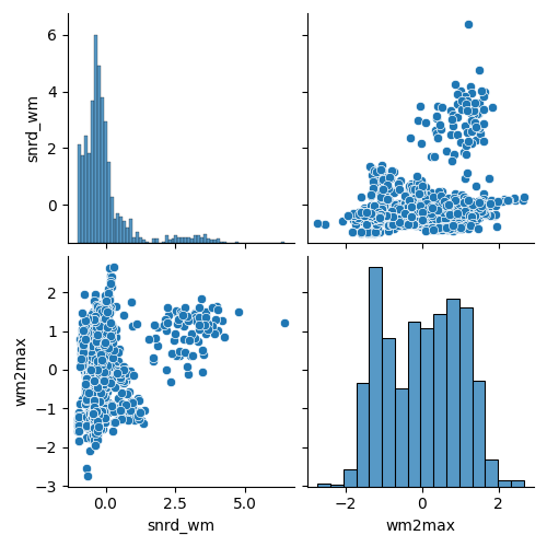
To gain an initial sense of how the IQMs relate to one another, we visualize their pairwise scatterplots. Because MRIQC provides a large number of IQMs, we display only a selected subset here.

import matplotlib.pyplot as plt
import seaborn as sns

sns.pairplot(iqms_scaled[iqms_scaled.columns[-2:]])

<seaborn.axisgrid.PairGrid object at 0x7f4267e93d10>

Interesting patterns emerge in the scatterplots: several IQMs show clear non‑linear relationships, which is important to keep in mind if linear dimensionality‑reduction methods struggle to capture the structure of the data. At the same time, many metrics are strongly correlated, underscoring how much redundancy exists within the full set of IQMs.

Feature selection¶

The redundancy among the IQMs makes the dataset especially suitable for feature selection, because many metrics capture overlapping aspects of image quality and therefore contribute similar information. Reducing the feature space helps isolate the dominant sources of variation and yields a more interpretable, lower‑dimensional representation of the data.

def greedy_uncorrelated(df, threshold=0.8):
    """
    Select a subset of approximately uncorrelated features from a DataFrame.

    This function iterates through the columns of the input DataFrame and
    greedily builds a set of features whose pairwise absolute correlations
    remain below a specified threshold. The first column is always selected,
    and each subsequent column is included only if it is sufficiently
    uncorrelated with all previously selected features.

    Parameters
    ----------
    df : pandas.DataFrame
        Input DataFrame containing the features to evaluate.
    threshold : float
        Maximum allowed absolute correlation between any pair of selected
        features. Columns with correlations above this value are excluded.
        Default is 0.8.

    Returns
    -------
    selected : list of str
        List of column names corresponding to the selected uncorrelated
        features.

    Notes
    -----
    This is a greedy algorithm: the order of columns in `df` affects the
    resulting selection.
    """
    corr_df = df.corr().abs()
    selected = []
    for col in corr_df.columns:
        if all(corr_df.loc[col, sel_col] < threshold for sel_col in selected):
            selected.append(col)
    return selected


uncorrelated = greedy_uncorrelated(iqms_scaled, threshold=0.45)
iqms_reduced = iqms_scaled[uncorrelated]
print(iqms_reduced)

          cjv       efc      fber  ...   snr_csf    snr_wm    wm2max
  0.859305 -0.859378 -0.208017  ...  1.084366 -1.689138 -0.268178
  1.408547  1.400283 -0.236468  ... -0.603625 -1.747567 -1.338395
  0.159444 -0.871493 -0.182213  ...  0.967272 -0.996662  1.052236
  1.158483 -0.749286 -0.206666  ...  1.168959 -1.449945  0.606781
  1.014771  0.576744 -0.234822  ... -1.767910 -1.531095 -1.592249
..        ...       ...       ...  ...       ...       ...       ...
-0.031305 -0.212088 -0.232681  ... -0.190341 -0.301485  0.714118
-0.175496 -0.185320 -0.231823  ...  0.723075  0.454689  0.645686
0.899248  0.566551 -0.235682  ...  0.178430 -1.332240  0.077362
-0.554522 -0.612112 -0.229016  ...  0.001251  0.713668  0.798304
0.755283  0.239425 -0.234451  ... -0.157003 -1.112779  0.293392

[1000 rows x 13 columns]

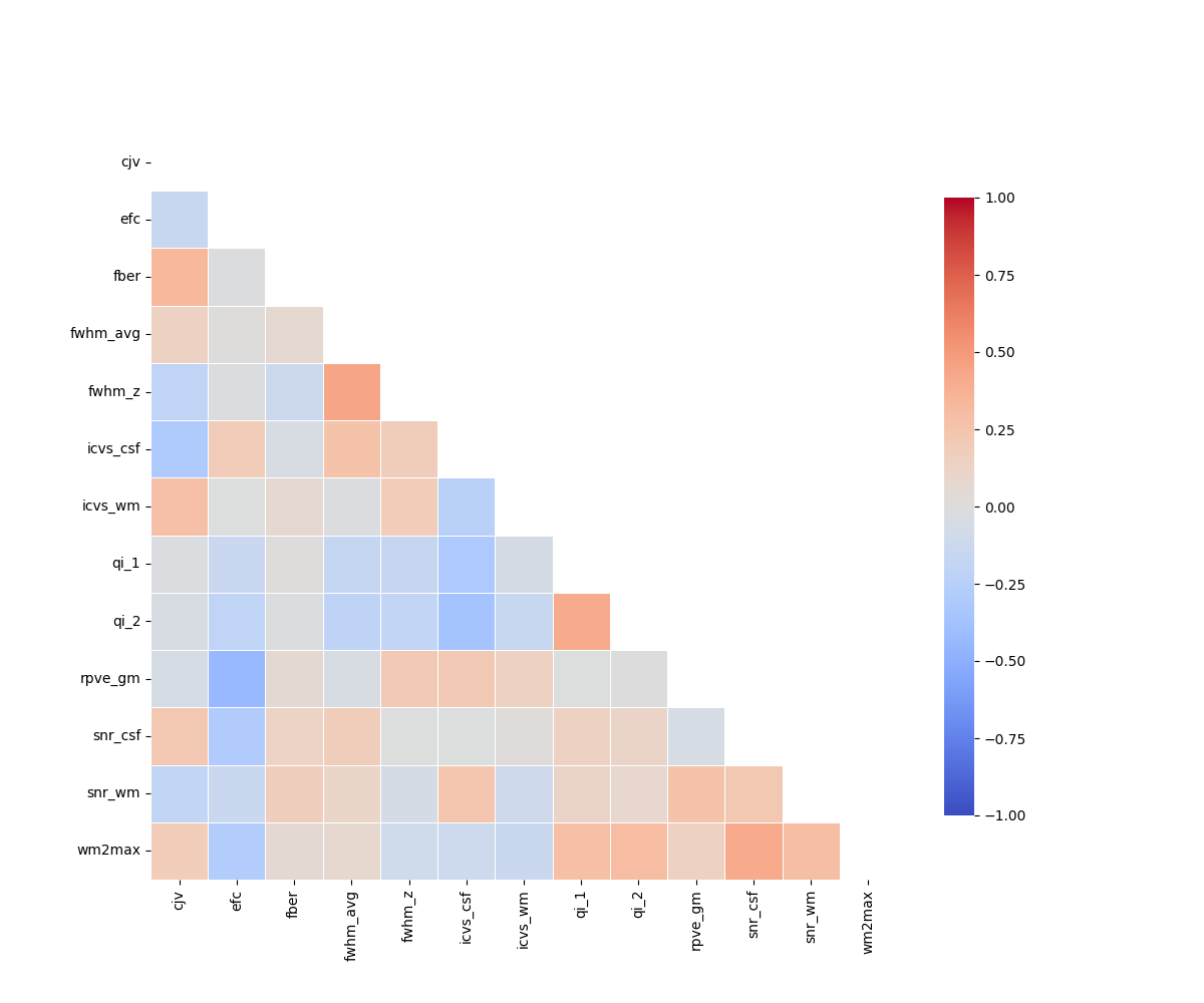
The metrics should not be too strongly correlated.

plt.figure(figsize=(12, 10))
corr = iqms_reduced.corr()
sns.heatmap(
    corr,
    mask=np.triu(np.ones_like(corr, dtype=bool), k=0),
    cmap="coolwarm",
    vmin=-1, vmax=1,
    square=True,
    linewidths=0.5,
    cbar_kws={"shrink": 0.8}
)

<Axes: >

Total running time of the script: (0 minutes 1.280 seconds)

Estimated memory usage: 129 MB

Gallery generated by Sphinx-Gallery